There may be times when we need to share an Excel file with others but we want to ensure that none of our data content gets altered in the process. Sometimes the people we share our spreadsheet files may assume it is okay to make changes or perhaps they make changes unintentionally and then save the changes to the same file name. These are just a couple of scenarios in which the ability to protect our sheets or even just specific cells within our sheet could be necessary.
In Excel 2016, we have options that allow us to protect our spreadsheet contents. What Excel actually allows us to do is to make our sheets or contents ?read-only? so that no changes can be saved to the protected parts of the file. In the following article, we will discuss just how to do this. All of our examples will be performed in Excel 2016 for Windows.
To get the most out of this guide, download the exercise file here and follow along.
Protecting your sheet
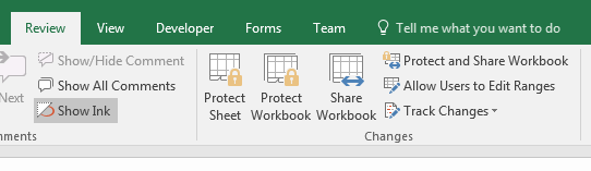
Let?s first take a look at how we can protect an entire worksheet so that our work does not get altered. The first thing we need to do select the ?Review? tab and in the ?Changes? group select ?Protect Worksheet?.

If you use the option to protect your sheet with a password be aware that there?s no ?I forgot my password? button in Excel. If you?re running Excel version 2007 or earlier Stellarinfo has software to recover your password.
If you?re running a newer version of Excel you?re out of luck.
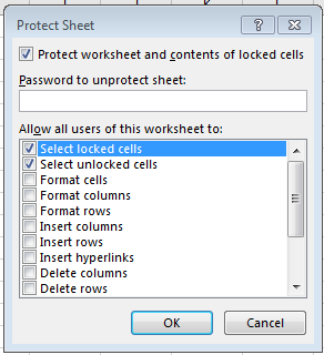

Click ?OK? and now the entire sheet will be protected from any kind of changes. If we try to enter any data into a cell or do any kind of copy/cut and paste operations, we will get a message alerting us to the fact that the worksheet is protected from any changes.
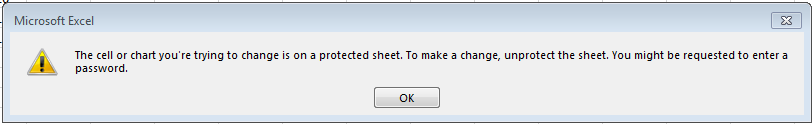

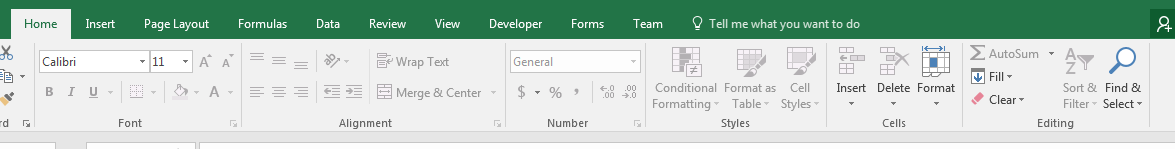
Any kind of edit will not be allowed as long as the worksheet is protected. Note the grayed out sections of the ribbon now that the worksheet is protected.

Protecting certain parts of your worksheet
Knowing how to protect an entire worksheet can certainly come in handy when we want to make sure anyone we share our workbook with doesn?t make any changes.
But what if we actually needed other users to add data to a part of a worksheet but not to make changes to other parts? In this case, we will need to protect certain cells but not the entire worksheet.
The technique to do this is pretty similar to what we just covered. What we need to do now is simply make a minor adjustment to allow users to edit cells in a range that we need them to while maintaining protection for other ranges.
Let’s say we have a table that users manually input a date in ‘mm/dd/yyyy’ format in the first column. Then our second and third columns contain formulas that take that input and output the original date data in ‘mmm-dd’ and ‘yyyy’
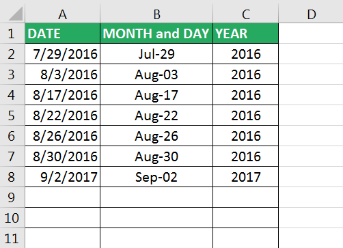

In this situation, we need to make sure our cells that contain the formulas are protected so they don’t get inadvertently changed by any of our data entry users. But we do want to make sure that the cells in the first column allow for changes in order for our users to input new data or make corrections to current data.
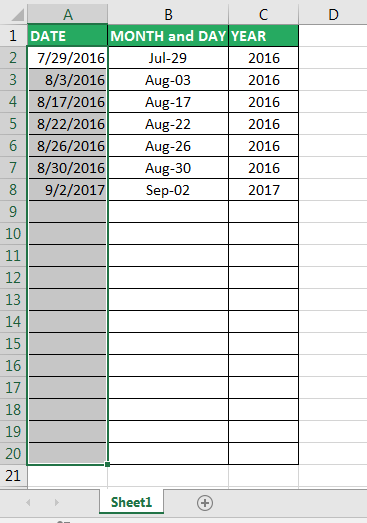
In order to do that, we just need to first make sure our sheet is not currently protected. Now we need to select the range we want to allow our users to edit (cells A2:A20).

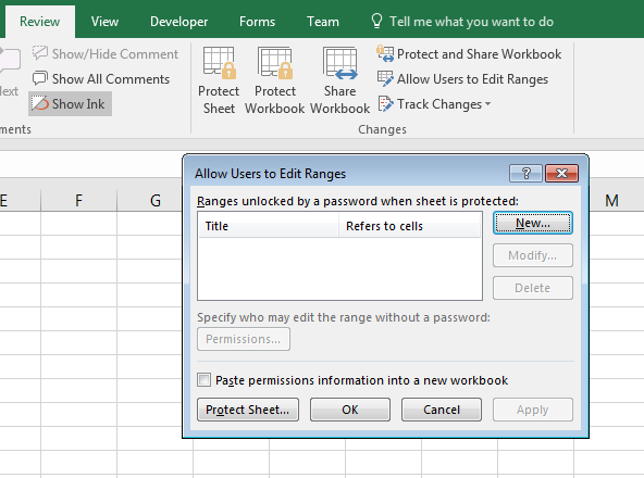
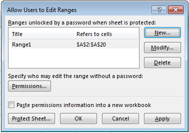
Then in the ‘Changes’ group on the ‘Review’ tab, click on ‘Allow Users to Edit Ranges’. A new window will open and now we need to click on the ‘New’ button.

The ‘New Range’ dialog box opens allowing us to name the new range and select the cells of the new range. This range should already be the range we pre-selected by default. If not, we can simply click into that box and re-select the range of our choosing.
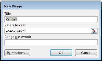

Again, Excel allows us to choose a password for access to this range if we would like but for this example, we will leave it blank and click ‘OK’. This returns us to the previous window and now the new range should appear with the title and cell range we selected. Click ‘Apply’ and then ‘OK’.

Then we simply need to protect the sheet like we did in our previous example. The sheet is now protected from any changes with the exception of our range that we have set to allow users to edit.
Now our users can enter new dates or revise old ones for the sake of correction. The formulas in our other columns are still functional but they cannot be changed, either unintentionally or otherwise.
Final thoughts
The example we have used in this article illustrates the perfect scenario where worksheet protection can be extremely useful. Furthermore, when we allow users the ability to edit only those ranges we set, we can control the integrity of things like formulas while not hindering the data entry functionality of a worksheet. Not only that, the ability to password protect sheets, and even editable ranges, provides even further flexibility to the owner of the worksheet.


